The picture below shows the required area between the two curves: y=e^(-x^2) (red) and y=1-cos(x) (blue). The vertical blue line shows the limit of the first quadrant (x=(pi)/2). Each grid square in the picture has an area of 0.04 and the area is roughly 14 complete squares: 14*0.04=0.56 is a rough estimate of the area between the curves.
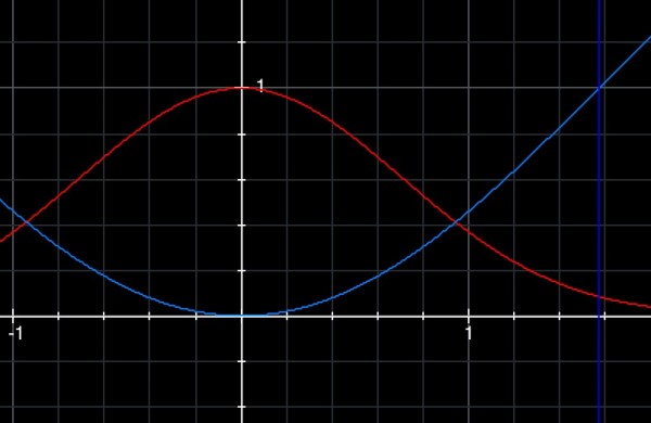
The points where the curves cross is the upper limit of the enclosed area which includes the y axis. I assume that the area beyond that up to x=(pi)/2 is not required because it is not enclosed by the y axis. The intersection is when x=0.941944 approx., that is, when e^(-x^2)=1-cos(x) (x in radians). At this point y=0.411783 approx. These define the upper limit for definite integration. Using S[low,high](...) to denote integration, we integrate to get the area between the two curves: S[0,0.941944]((e^(-x^2)-1+cos(x))dx).
As far as I know, there's no solution to the indefinite integral of e^(-x^2), but the above definite integral can be evaluated by approximating dx. If dx=0.01, for example, then we can sum the areas of thin rectangles of width 0.01 over the range. This is tedious but it will yield a reasonable approximation.
Let f(x)=e^(-x^2)-1+cos(x). Consider a starting point represented by a rectangle of width 0.01 and height f(0). Its area is 1*0.01=0.01. Now consider a different rectangle with the same width but height f(0.01) and area=0.0099985. The two rectangles "trap" the curve between them, so the true area under the curve between the limits 0 and 0.01 is somewhere between the two rectangular areas. If we take the average of these two areas we get 0.00999925.
Then we move to f(0.01) and f(0.02). The two areas this time are 0.01f(0.01) and 0.01f(0.02) and the average area is 0.005(f(0.01)+f(0.02)). A third pair of rectangles will be averaged at 0.005(f(0.02)+f(0.03)). The last pair of rectangles will be narrower than 0.01: the first has a height of f(0.94) and a width of 0.001944, the second has a height of f(0.941944) which approximates to zero (to the nearest 10^-7). So the last average area is 0.000972f(0.94).
The total area between the curves and the y axis can be expressed as a series:
0.005(f(0)+f(0.01) + f(0.01)+f(0.02) + ... + f(0.92)+f(0.93) + f(0.93)+f(0.94)) + 0.000972f(0.94).
As you can see, f(0.01) to f(0.93) are all repeated, so we have 0.005(f(0)+f(0.94)) + 0.000972f(0.94) + 0.01(f(0.01)+...+f(0.93)). Since f(0)=1 and f(0.94)=).00308040 approx. So the first expression is 0.005*1.00308040=0.0050154020. 0.000972f(0.94)=0.000972*0.00308040=0.000003 approx.
To make matters more manageable, I'll divide the range of values into summed groups: 0.01-0.10, 0.11-0.20, 0.21-0.30, etc., up to 0.81-0.90, then 0.91-0.94.
Here are the group results (these figures have a superfluous accuracy and will be rounded off later):
0.01-0.10: 9.946463769
0.11-0.20: 9.630991473
0.21-0.30: 9.036361176
0.31-0.40: 8.183088444
0.41-0.50: 7.104969671
0.51-0.60: 5.842140126
0.61-0.70: 4.437880465
0.71-0.80: 2.935475192
0.81-0.90: 1.375462980
0.91-0.93: 0.104328514
TOTAL: 58.59716181 AREA SUBTOTAL: 0.5859716181 TOTAL AREA: 0.585972+0.005018=0.591 approx.
Control summation: 5.415713508. Control area subtotal: 0.5415713508 (based on increments of 0.1 across the range 0.1 to 0.9. We would expect this figure to be approximately the same as the more accurate summation.)
It appears that the area between the curves and the y axis is of the order 0.591; this figure is close to the rough estimate given near the beginning of this answer.