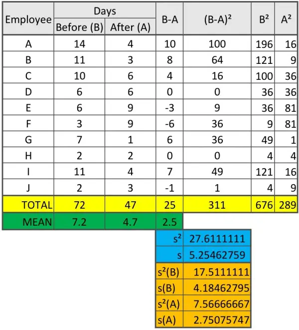
In the table, Before and After refer to the introduction of the incentive program. Some statistics have been calculated from the data. The target data is the difference between the before and after values.
The sample variance, s² = (∑(B-A)²-(∑(B-A)²)/n)/(n-1) where n=10, the sample size.
From this the sample SD is the square root of the variance.
From t tables with 9 DOF, we read a value of 2.262 (2-tail because we are considering a range below and above the mean difference). This tell us how far from the mean is the standard deviation for a 95% CI. But we have to adjust s to s/√n=5.2546/√10=1.662 approx.
Answer to part 1:
The CI is 2.5±2.262×1.662=2.5±3.76, giving us the interval:
-1.26≤mean difference≤6.26 days. This can be written [-1.26,6.26].
So, the mean difference between the average number of days lost before and after introduction of the incentive program lies between -1.26 and 6.26 days.
Answer to part 2:
CONDITION CHECK
See comment.
CLAIM
The incentive program reduces the number of days lost.
HYPOTHESES
Without the incentive program, no difference would be expected so H0: mean difference=0.
The incentive program was designed to reduce the absenteeism so H1: A<B, A-B<0, or B-A>0, mean difference is B-A, so mean difference>0. This implies a one-tailed t test.
p-VALUE
t=2.5/1.662=1.504, corresponding to a p-value of 0.0834. (9 DOF, 1-tail test 0.05 is implied.) Compared to significance level of 0.05. The p-value is not more extreme than the required significance level.
CONCLUSION
See comment.
More to follow...