Question

Compute the least squares regression line of Y on X for the following data:

X	5	6	8	10	12
Y	16	19	23	28	36

1. What is the regression co-efficient and what does it mean?
 2. Find the predicted values of Y for X= 15 & 20. 

Answer 1

 

X	Y	XY	X2	Y2
05	016	0080	025	0256
06	019	0114	036	0361
08	023	0184	064	0529
10	028	0280	100	0784
12	036	0432	144	1296
41	122	1090	369	3226

(Extra zeroes have been inserted to make addition easier visually.)

This table enables m and b to be calculated where Y=mX+b. m is the line gradient in this linear regression and b is the Y-intercept.

The last row in the table is the sum of the column values, where sum is indicated by ∑ in the formulas.

m=(n∑XY-∑X∑Y)/(n∑X²-(∑X)²), b=(∑Y-m∑X)/n, where n=5 (the data size).

Now we can plug in values from the table:

m=(5×1090-41×122)/(5×369-41²)=(5450-5002)/(1845-1681)=448/164=2.73 approx.

b=(122-(448/164)41)/5=2.

So Y=2.73X+2.

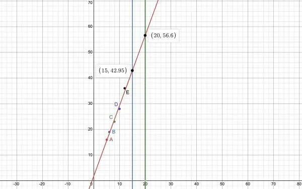
The given points are labelled A-E. The intersections (X,Y) of the blue and green vertical lines with the best fit line (linear regression) reveal the required values for part 2. 

1. Regression coefficient r=0.991 approx. It's clear that the regression coefficient r is close to 1 because the red line is very close to the given points. r close to 1 means that the points are almost in a straight line. r close to zero means that there's very little correspondence of the X and Y values.

This is calculated from the formula r=(n∑xy-∑x∑y)/(√[(n∑x²-(∑x)²)(n∑y²-(∑y)²)]. 

2. X=15, Y=42.95 (43); X=20, Y=56.6 (57). So the predicted values of Y are about 43 and 57 (nearest integers).